Beyond the Shocks: Shape-Preserving Reconstruction in 2D Data Flows

The Problem: Accuracy vs. Monotonicity ⚖️

In the univariate case, reconstructing data with $C^1$ discontinuities (jumps) is a well-understood challenge. However, it presents a classic mathematical trade-off: Accuracy vs. Monotonicity.

The real trade-off: Regions with enforced monotonicity constraints typically correspond to lower formal accuracy, and vice versa.

In other words, if we push for high-order accuracy (perhaps needing a sharper image in a specific region), we often trigger non-physical oscillations. Conversely, if we enforce strict monotonicity, we risk losing the fine details of the signal.

To address this, my research focused on extending 1D properties to the bivariate case. The choice, made at the very beginning, was to adopt Cubic Hermite Interpolators for two main reasons:

Industrial Standard: These interpolants are a cornerstone in fields like Computational Fluid Dynamics (CFD) and Computer-Aided Design (CAD) for managing discontinuities while preserving the data’s physical shape. 🛠️
Derivative Approximation: By construction, these interpolants depend heavily on how derivatives are approximated. This allows for a “building-block” approach: adopting different non-linear means to approximate derivatives and—voilà—you have your shape-preserving reconstruction.

🌀 Moving to 2D: The “Curse” of Dimensionality

As with almost every problem in mathematics, increasing the dimension often destroys the “nice” properties found in lower dimensions. In the bivariate case, finding necessary and sufficient conditions for monotonicity is both computationally and theoretically daunting.

My research specifically focused on:

Extension: Mapping 1D monotonicity properties onto 2D grids.
Algorithm Development: Creating different derivative estimators to ensure a reliable, artifact-free reconstruction.

I explored the reconstruction of images and general data flows, aiming for interpolants that are monotone-preserving to eliminate phenomena such as Gibbs oscillations (spurious oscillations). 🚫〰️

📊 Experimental Results

The following figures illustrate the core of my research results:

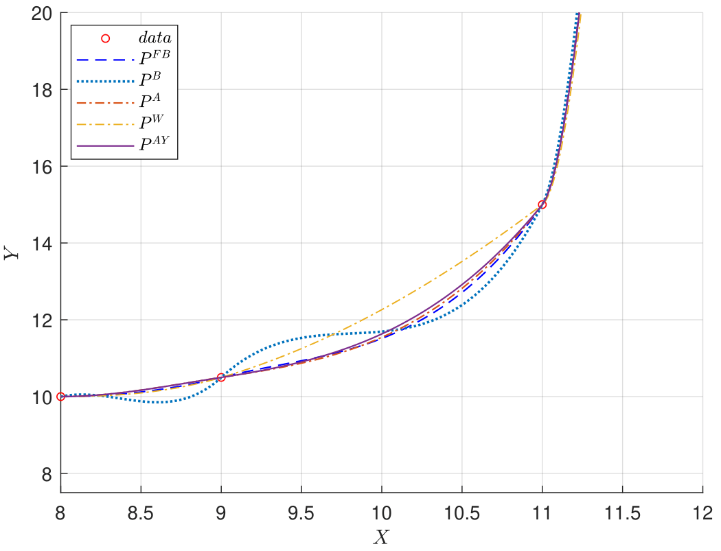
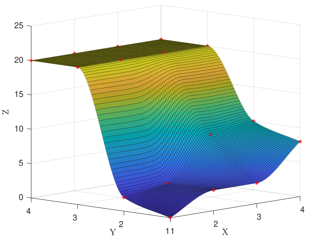
1D Case — **1. Univariate Case:** Diverse non-linear estimators used to reconstruct a function with a jump.

2D Case — **2. Bivariate Case:** Monotone-preserving reconstruction of a 2D surface.

These images represent the practical outcome of the algorithms I developed: on the left, you can see how different estimators behave under “stress” (jumps), while on the right, the 2D surface remains clean and stable, completely free from the typical “ringing” artifacts that usually plague high-order methods.

⚡ From Linear Limits to Non-Linear Resilience

As mentioned The first approach—justifiably trivial—is to implement linear means, such as the standard arithmetic mean or the geometric mean. However, numerical literature provides robust evidence that linear schemes are strictly limited in their accuracy when dealing with discontinuities; according to Godunov’s Theorem, linear schemes that preserve monotonicity are at most first-order accurate. This “glass ceiling” of accuracy makes it natural to pivot toward more sophisticated non-linear means.

In the 1D comparison charts above, we tested various linear and non-linear estimators. When faced with “wild” data, the weaker linear models fail predictably. To bridge this gap, we seek non-linear means that maintain high-order accuracy while strictly enforcing shape-preserving constraints.

Many real-world applications require reconstructions that preserve specific geometric properties, such as convexity or monotonicity. Let’s draw a financial parallel to highlight the practical impact: Imagine reconstructing the price action or volatility of a stock. If the data undergoes a sudden “shock”—a massive jump in value—an imprecise, low-quality interpolant will trigger spurious oscillations (ringing artifacts). These fluctuations suggest market volatility that doesn’t actually exist, leading to catastrophic errors in automated trading or risk assessment. In short: if your math cannot handle the jump, it invents a reality that isn’t there.

🌀 The “Curse” of the Second Dimension: A Topological Grid-lock

Moving to the bivariate case, the core problem remains identical, but the geometric complexity scales exponentially. As is often the case in mathematics, increasing the dimension often destroys what was discovered or achieved “on the lower floors.” The difficulties here are twofold:

Topological Rigidity: In 1D, monotonicity is a simple “left-to-right” constraint within a single interval. In 2D, we lose this total ordering. A point on a surface is constrained by its neighbors in every direction ($x$, $y$, and diagonally). This creates a topological “grid-lock” where enforcing a constraint in one direction can inadvertently trigger an oscillation in another, making it theoretically daunting to find a universal non-linear mean that works across the entire manifold.
Derivative Approximation: In 2D, we must approximate partial derivatives $\partial_x$ and $\partial_y$ which were not present in 1D. This process is inherently difficult because the accuracy of the entire surface depends on how these slopes are estimated at the boundaries of each cell. More details in the following section.

📐 Formal Definition: The Piecewise Bicubic Hermite Polynomial

To ground our discussion in mathematical rigor, let us define the interpolant on a rectangular domain. Given a grid cell $\Omega_{i,j} = [x_i, x_{i+1}] \times [y_j, y_{j+1}]$, the Piecewise Bicubic Hermite Interpolant $S(x, y)$ is the unique polynomial that matches the function values, first-order partial derivatives, and mixed partial derivatives (the “twist” terms) at the four corners of the cell.

Using the local normalized coordinates $u = \frac{x - x_i}{h_x}$ and $v = \frac{y - y_j}{h_y}$ (where $u, v \in [0, 1]$), the functional form is expressed through the Kronecker product of univariate cubic Hermite basis functions:

$$ \begin{aligned} S(x, y) = \sum_{i=0}^1 \sum_{j=0}^1 \Big[ & f_{i,j} \mathcal{H}_i(u) \mathcal{H}_j(v) + \partial_x f_{i,j} \mathcal{G}_i(u) \mathcal{H}_j(v) + \\ & \partial_y f_{i,j} \mathcal{H}_i(u) \mathcal{G}_j(v) + \partial_{xy} f_{i,j} \mathcal{G}_i(u) \mathcal{G}_j(v) \Big] \end{aligned} $$

In this formulation, $\mathcal{H}_k$ and $\mathcal{G}_k$ are the cardinal cubic splines that satisfy the Hermite conditions. While the 1D case is a straightforward $C^1$ cubic spline, the 2D transition introduces a significant jump in complexity:

The Twist Term ($\partial_{xy} f_{i,j}$): This mixed derivative represents the rate of change of the $x$-slope in the $y$-direction. In many standard libraries, this term is set to zero or approximated linearly, often leading to “flat” spots or non-physical ripples.
The “Final Boss” of Numerical Stability: Approximating these cross-derivatives while maintaining monotonicity is the core challenge. An incorrect estimation of $\partial_{xy}$ is the primary cause of surface distortion; it is the mathematical “glitch” that destroys the shape-preserving property we worked so hard to achieve on the 1D “lower floors.”

💡 Final Thoughts: Why This Matters

This research isn’t just about “cleaner” graphs. In a world driven by data, the ability to preserve the integrity of a signal during reconstruction is vital. Whether it’s medical imaging, satellite data, or anomaly detection in cybersecurity, the math remains the same: distinguishing the real shock from the numerical noise. 🚀